Recall that in the lessons on numpy arrays, you ran multiple functions to get the mean, minimum and maximum values of numpy arrays. This fast calculation of summary statistics is one benefit of using pandas dataframes. You have now learned how to run calculations and summary statistics on columns in pandas dataframes.

On the next page, you will learn various ways to select data from pandas dataframes, including indexing and filtering of values. It is a data structure where data is stored in tabular form. Datasets are arranged in rows and columns; we can store multiple datasets in the data frame. We can perform various arithmetic operations, such as adding column/row selection and columns/rows in the data frame. For example, you used .shape to get the structure (i.e. rows, columns) of a specific numpy array using array.shape. This attribute .shape is automatically generated for a numpy array when it is created.
You can use the method .info() to get details about a pandas dataframe (e.g. dataframe.info()) such as the number of rows and columns and the column names. Once you have a dataset stored as a matrix or dataframe in R, you'll want to start accessing specific parts of the data based on some criteria. For example, if your dataset contains the result of an experiment comparing different experimental groups, you'll want to calculate statistics for each experimental group separately. The process of selecting specific rows and columns of data based on some criteria is commonly known as slicing. In this chapter, you will explore some methods (i.e. functions specific to certain objects) that are accessible for pandas dataframes. At the start of every analysis, data needs to be cleaned, organised, and made tidy.

For every Python Pandas DataFrame, there is almost always a need to delete rows and columns to get the right selection of data for your specific analysis or visualisation. The Pandas Drop function is key for removing rows and columns. The second most common requirement for deleting rows from a DataFrame is to delete rows in groups, defined by values on various columns. The best way to achieve this is through actually "selecting" the data that you would like to keep. The "drop" method is not as useful here, and instead, we are selecting data using the "loc" indexer and specifying the desired values in the column we are using to select. Indexing dataframes with logical vectors is almost identical to indexing single vectors.

First, we create a logical vector containing only TRUE and FALSE values. Next, we index a dataframe using the logical vector to return only values for which the logical vector is TRUE. A pandas dataframe is a tabular structure with rows and columns. One of the most popular environments for performing data-related tasks is Jupyter notebooks. In Jupyter notebooks, the dataframe is rendered for display using HTML tags and CSS. This means that you can manipulate the styling of these web components.

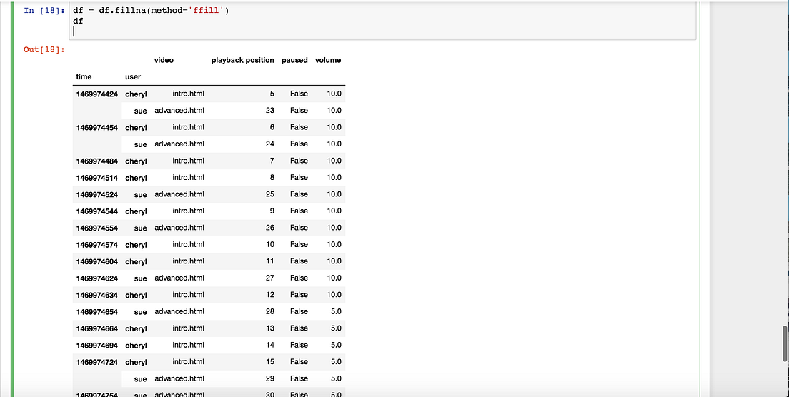
You can also use the attribute .columns to see just the column names in a dataframe, or the attribute .shape to just see the number of rows and columns. Begin by importing the necessary Python packages and then downloading and importing data into pandas dataframes. Pandas documentation provides a list of all attributes and methods of pandas dataframes. The DataFrame index is displayed on the left-hand side of the DataFrame when previewed.

To delete rows from a DataFrame, the drop function references the rows based on their "index values". Most typically, this is an integer value per row, that increments from zero when you first load data into Pandas. You can see the index when you run "data.head()" on the left hand side of the tabular view. You can access the index object directly using "data.index" and the values through "data.index.values". This dataset contains 5,000 rows, which were sampled from a 500,000 row dataset spanning the same time period.

In this case, a sample is fine because our purpose is to learn methods of data analysis with Python, not to create 100% accurate recommendations to Watsi. Because logical subsetting allows you to easily combine conditions from multiple columns, it's probably the most commonly used technique for extracting rows out of a data frame. You'll then learn how those six ways act when used to subset lists, matrices, and data frames. Let's understand another example to create dataframe by passing lists of dictionary and rows. We can pass the lists of dictionaries as input data to create the Pandas dataframe. In this chapter, you will use attributes (i.e. metadata) to get more information about pandas dataframes that is automatically generated when it is created.

The group_by() function in dplyr allows you to perform functions on a subset of a dataset without having to create multiple new objects or construct for()loops. The combination of group_by() and summarise() are great for generating simple summaries of grouped data. When you have repeating columns names, a safe method for column removal is to use the iloc selection methodology on the DataFrame. In this case, you are trying to "select all rows and all columns except the column number you'd like to delete". We can select specific ranges of our data in both the row and column directions using either label or integer-based indexing. Let's understand another example to create the pandas dataframe from list of dictionaries with both row index as well as column index.

I'd be interested in any element of removing rows or columns not covered in the above tutorial – please let me know in the comments. The drop function can be used to delete columns by number or position by retrieving the column name first for .drop. To get the column name, provide the column index to the Dataframe.columns object which is a list of all column names. By default Jupyter Notebook will limit the number of rows and columns when displaying a data frame to roughly fit the screen size . When selecting a column, you'll use data[], and when selecting a row, you'll use data.iloc[] or data.loc[].

To learn more about the differences between .iloc and .loc, check out pandas documentation. The datasets object is a list, where each item is a DataFrame corresponding to one of the SQL queries in the Mode report. So datasets is a dataframe object within the datasets list. You can see that the above command produces a table showing the first 5 rows of the results of your SQL query.

We will use python's list comprehensions to create lists of the attribute columns in the DataFrame, then print out the lists to see the names of all the attribute columns. DataFrames are table-like structures comprised of rows and columns. In relational database, SQL joins are fundamental operations that combine columns from one or more tables using values that are common to each. It also saves the readme file, explanations of variables, and validation metadata, and combines these all into a single 'list' that we called 'loadData'. The only part of this list that we really need for this tutorial is the 'mam_pertrapnight' table, so let's extract just that one and call it 'myData'.

Removing columns and rows from your DataFrame is not always as intuitive as it could be. The drop function allows the removal of rows and columns from your DataFrame, and once you've used it a few times, you'll have no issues. The url column you got back has a list of numbers on the left. This is called the index, which uniquely identifies rows in the DataFrame. You will use the index to select individual rows, similar to how you selected rows from a list in an earlier lesson.

A unique identifier is often necessary to refer to specific records in the dataset. For example, the DMV uses license plates to identify specific vehicles, instead of "Blue 1999 Honda Civic in California," which may or may not uniquely identify a car. Nested inside this list is a DataFrame containing the results generated by the SQL query you wrote. To learn more about how to access SQL queries in Mode Python Notebooks, read this documentation. Let's create two logical vectors and their integer equivalents, and then explore the relationship between Boolean and set operations.

Indexing with brackets is the standard way to slice and dice dataframes. Let's look at how joins work with dataframes by using subsets of our original DataFrame and the pandas merge fucntionality. We'll then move onto examining a spatial join to combine features from one dataframe with another based on a common attribute value. In addition to row and column indices to search a DataFrame, we can use a spatial indexes to quickly access information based on its location and relationship with other features. They are based on the concept of a minimum bounding rectangle - the smallest rectangle that contains an entire geometric shape. Access to points, complex lines and irregularly-shaped polygons becomes much quicker and easier through different flavors of spatial indexing.
In this detailed article, we saw all the built-in methods to style the dataframe. Then we looked at how to create custom styling functions and then we saw how to customize the dataframe by modifying it at HTML and CSS level. We also saw how to save our styled dataframe into excel files. Pandas DataFrame can be created by passing lists of dictionaries as a input data. The dict of ndarray/lists can be used to create a dataframe, all the ndarray must be of the same length.

The index will be a range by default; where n denotes the array length. We can create dataframe using a single list or list of lists. In this tutorial, we will learn to create the data frame in multiple ways. We often need to get a subset of data using one function, and then use another function to do something with that subset .
This leads to nesting functions, which can get messy and hard to keep track of. Enter 'piping', dplyr's way of feeding the output of one function into another, and so on, without the hassleof parentheses and brackets. When working with data frames in R, it is often useful to manipulate and summarize data. The dplyr package in R offers one of the most comprehensive group of functions to perform common manipulation tasks. In addition, thedplyr functions are often of a simpler syntax than most other data manipulation functions in R. If you .iloc, it will return to you the row at the 1st index regardless of the index's name.

In the case of this dataframe .iloc and .loc will return the same row. To select a specific row, you must use the .iloc or .loc method, with the row's index in brackets. Then, let's say we want to duplicate the info table so that we have a row for each value in grades. An elegant way to do this is by combining match() and integer subsetting (match returns the position where each needle is found in the haystack). The document will also demonstrate spatial joins to combine dataframes.

Like every image has a caption that defines the post text, you can add captions to your dataframes. This text will depict what the dataframe results talk about. They may be some sort of summary statistics like pivot tables. For now, let's create a sample dataset and display the output dataframe. The operation is quite complicated and involves reading and manipulating various datasets which ultimate results in one number being generated.
I want to add that number into the correct row in my existing dataframe. For example, you could group the example dataframe by the seasons and then run the describe() method on precip. This would run .describe() on the precipitation values for each season as a grouped dataset.

In this example, the label_column on which you want to group data is seasons and the value_column that you want to summarize is precip. If column_name_2 already exists, then the values are replaced by the calculation (e.g. values in column_name_2 are set to values of column_name_1 divided by 25.4). If column_name_2 does not already exist, then the column is created as the new last column of the dataframe. Note that using the double set of brackets [] around column_name selects the column as a dataframe, and thus, the output is also provided as a dataframe. The output of .describe() is provided in a nicely formatted dataframe.

Note that in the example dataset, the column called precip is the only column with numeric values, so the output of .describe() only includes that column. This is read as "from data frame myMammalData, select only males and return the mean weight as a new list mean_weight". The subsequent arguments describe how to manipulate the data (e.g., based on which columns, using which summary statistics), and you can refer to columns directly (without using $).

It can be useful for selection and aggregation to have a more meaningful index. For our sample data, the "name" column would make a good index also, and make it easier to select country rows for deletion from the data. To remove columns using iloc, you need to create a list of the column indices that you'd like to keep, i.e. a list of all column numbers, minus the deleted ones. The default way to use "drop" to remove columns is to provide the column names to be deleted along with specifying the "axis" parameter to be 1. The Pandas "drop" function is used to delete columns or rows from a Pandas DataFrame. The brackets selecting the column and selecting the rows are separate, and the selections are applied from left to right .

Through their website, Watsi enables direct funding of medical care. Take the time to understand what that looks like in practice. Visit some of the URLs you see in this dataset to familiarize yourself with the structure of the site and content, such as Mary's patient profile.

Google Watsi and consider why people might engage with the service. Context is important - it'll help you make educated inferences in your analysis of the data. It's similar in structure, too, making it possible to use similar operations such as aggregation, filtering, and pivoting.

However, because DataFrames are built in Python, it's possible to use Python to program more advanced operations and manipulations than SQL and Excel can offer. As a bonus, the creators of pandas have focused on making the DataFrame operate very quickly, even over large datasets. Subsetting a list works in the same way as subsetting an atomic vector. Using [ always returns a list; [[ and $, as described in Section 4.3, let you pull out elements of a list. This is not useful for 1D vectors, but, as you'll see shortly, is very useful for matrices, data frames, and arrays. To illustrate, I'll apply [ to 1D atomic vectors, and then show how this generalises to more complex objects and more dimensions.

The rows where the on parameter value is the same in both tables have all attributes from both DataFrames in the result. The rows from the first DataFrame that do not have a matching NAME value in the second dataframe have values filled in with NaN values. The POP2010 attribute from the left DataFrame is combined with all the attributes from the right DataFrame. A Spatial join is a table operation that affixes data from one feature layer's attribute table to another based on a spatial relationship. The spatial join involves matching rows from the Join Features to the Target Features based on their spatial relationship.

As GIS analysts and data scientists, we also want to query based on geographic location. We can do that by building a spatial index with the sindex property of the spatial dataframe. The resulting quadtree index allows us to query based on specific geometries in relation to other geometries.

The DataFrame.info() provides a concise summary of the object. This method prints information about a DataFrame including the index dtype and column dtypes, non-null values and memory usage. As mentioned in the Introduction to the Spatially Enabled DataFrame guide, the Pandas DataFrame structure underlies the ArcGIS API for Python's Spatially Enabled DataFrame. Each of these axes are indexed and labeled for quick and easy identification, data alignment, and retrieval and updating of data subsets. We are using the Boolean object pd.isnull(surveys_df['weight']) as an index to surveys_df. We are asking Python to select rows that have a NaN value of weight.